Research is what I'm doing when I don't know what I'm doing.
Wernher von Braun
Welcome to the second instalment of our second series on Computational Neuroscience for lay people. You can find the first post of the previous series here, and the first post of the current series here. As you'd expect, this second series is slightly more advanced, and, as such, it is peppered with unavoidable technical jargon. Having said that, we shall continue to pursue our ambitious target of making things as easy to parse as possible (but no easier). If you read the first series, the second should hopefully make some sense.1
Our last post discussed Computational Neuroscience as a discipline, and the kind of things one may want to do in this field. We also spoke about models and their composition, and the desirable properties of a platform that runs simulations of said models. However, it occurred to me that we should probably build some kind of "end-to-end" understanding; that is, by starting with the simulations and models we are missing a vital link with the physical (i.e. non-computational) world. To put matters right, this part attempts to provide a high-level introduction on how data is acquired from the real world and can then be used - amongst other things - to inform the modeling process.
Macro and Micro Microworlds
For the purposes of this post, the data gathering process starts with the microscope. Of course, keep in mind that we are focusing only on the morphology at present - the shape and the structures that make up the neuron - so we are ignoring other important activities in the lab. For instance, one can conduct experiments to measure voltage in a neuron, and these measurements provide data for the functional aspects of the model. Alas, we will skip these for now, with the promise of returning to them at a later date2.
So, microscopes then. Microscopy is the technical name for the observation work done with the microscope. Because neurons are so small - some 4 to 100 microns in size - only certain types of microscopes are suitable to perform neuronal microscopy. To make matters worse, the sub-structures inside the neuron are an important area of study and they can be ridiculously small: a dentritic spine - the minute protrusions that come out of the dendrites - can be as tiny as 500 nanometres; the lipid bylayer itself is only 2 or 3 nanometres thick, so you can imagine how incredibly small ion channels and pumps are. Yet these are some of the things we want to observe and measure. Lets call this the "micro" work. On the other hand, we also want to understand connectivity and other larger structures, as well as perform observations of the evolution of the cell and so on. Lets call this the "macro" work. These are not technical terms, by the by, just so we can orient ourselves. So, how does one go about observing these differently sized microworlds?

Figure 1: Example of measurements one may want to perform on a dendrite. Source: Reversal of long-term dendritic spine alterations in Alzheimer disease models
Optical Microscopy
The "macro" work is usually done using the Optical "family" of microscopes, which is what most of us think of when hearing the word microscope. As it was with Van Leeuwenhoek's tool in the sixteen hundreds, so it is that today's optical microscopes still rely on light and lenses to perform observations. Needless to say, things did evolve a fair bit since then, but standard optical microscopy has not completely removed the shackles of its limitations. These are of three kinds, as Wikipedia helpfully tells us: a) the objects we want to observe must be dark or strongly refracting - a problem, since the internal structures of the cell are transparent; b) visible light's diffraction limit means that we cannot go much lower than 200 nanometres - pretty impressive, but unfortunately not quite low enough for detailed sub-structure analysis; and c) out of focus light hampers image clarity.
Workarounds to these limitations have been found in the guise of techniques, with the aim of augmenting the abilities of standard optical microscopy. There are many of these techniques. There is the Confocal Microscopy3 - improving resolution and contrast; the Fluorescence microscope, which uses a sub-diffraction technique to reconstruct some of the detail that is missing due to diffraction; or the incredible-looking movies produced by Multiphoton Microscopy. And of course, it is possible to combine multiple techniques in a single microscope, as is the case with the Multiphoton Fluorescence Microscopes (MTMs) and many others.
In fact, given all of these developments, it seems there is no sign of optical microscopy dying out. Presumably some of this is due to the relative lower cost of this approach as well as to the ease of use. In addition, optical microscopy is complementary to the other more expensive types of microscopes; it is the perfect tool for "macro" work that can then help to point out where to do "micro" work. For example, you can use an optical microscope to assess the larger structures and see how they evolve over time, and eventually decide on specific areas that require more detailed analysis. And when you do, you need a completely different kind of microscope.
Electron Microscopy
When you need really high-resolution, there is only one tool to turn to: the Electron Microscope (EM). This crazy critter can provide insane levels of magnification by using a beam of electrons instead of visible light. Just how insane, you ask? Well, if you think that an optical microscope lives in the range of 1500x to 2000x - that is, can magnify a sample up to two thousand times - an EM can magnify as much as 10 million times, and provide a sub-nanometre resolution4. It is mind boggling. If fact, we've already seen images of atoms using EM in part II, but perhaps it wasn't easy to appreciate just how amazing a feat that is.
Of course, EM is itself a family - and a large one at that, with many and diverse members. As with optical microscopy, each member of the family specialises on a given technique or combination of techniques. For example, the Scanning Electron Microscope (SEM) performs a scan of the object under study, and has a resolution of 1 nanometre or higher; the Scanning Confocal Electron Microscope (SCEM) uses the same confocal technique mentioned above to provide higher depth resolution; and Transmission Electron Microscopy (TEM) has the ability to penetrate inside the specimen during the imagining process, given samples with thickness of 100 nanometres or less.
A couple of noteworthy points are required at this juncture. First, whilst some of these EM techniques may sound new and exciting, most have been around for a very long time; it just seems they keep getting better and better as they mature. For example, TEM was used in the fifties to show that neurons communicate over synaptic junctions but its still wildly popular today. Secondly, its important to understand that the entire imaging process is not at all trivial - certainly not for TEM, nor EM in general and probably not for Optical Microscopy either. It just is a very labour intensive and very specialised process - most likely done by an expert human neuroanatomist - and the difficulties range from the chemical preparation of the samples all the way up to creating the images. The end product may give the impression it was easy to produce, but easy it was not.
At any rate, whatever the technical details, the fact is that the imagery that results from all these advances is truly evocative - haunting, even. Take this image produced by SEM:
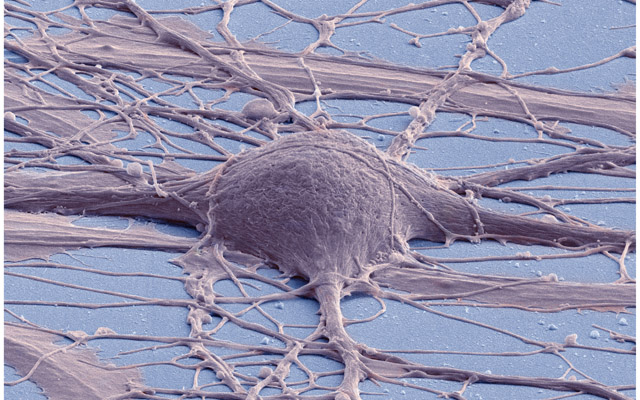
Figure 2: Human neuron. Source: New Reprogramming Method Makes Better Stem Cells
Personally, I think it is incredibly beautiful; simultaneously awe-inspiring and depressing because it really conveys the messiness and complexity of wetware. By way of contrast, look at the neatness of man-made micro-structures:

Figure 3: The BlueGene/Q chip. Source: IBM plants transactional memory in CPU
Stacks and Stacks of 'Em
Technically, pictures like the ones above are called micrographs. As you can see in the neuron micrograph, these images provide a great visual description of the topology of the object we are trying to study. You also may notice a slight coloration of the cell in that picture. This is most likely due to the fact that the people doing the analysis stain the neuron to make it easier to image. Now, in practice - at least as far as I have seen, which is not very far at all, to be fair - 2D grayscale images are preferred by researchers to the nice, Public Relations friendly pictures like the one above; those appear to be more useful for magazine covers. The working micrographs are not quite as exciting to the untrained eye but very useful to the professionals. Here's an example:

Figure 4: The left-hand side shows the original micrograph. On the right-hand side it shows the result of processing it with machine learning. Source: Deep Neural Networks Segment Neuronal Membranes in Electron Microscopy Images
Let's focus on the left-hand side of this image for the moment. It was taken using ssTEM - serial-section TEM, an evolutionary step in TEM. The ss part of ssTEM is helpful in creating stacks of images, which is why you see the little drawings on the left of the picture; they are there to give you the idea that the top-most image is one of 30 in a stack5. The process of producing the images above was as follows: they started off with a neuronal tissue sample, which is prepared for observation. The sample had 1.5 micrometres and was then sectioned into 30 slices of 50 nanometres. Each of these slices was imaged, at a resolution of 4x4 nanometres per pixel.
As you can imagine, this work is extremely sensitive to measurement error. The trick is to ensure there is some kind of visual continuity between images so that you can recreate a 3D model from the 2D slices. This means for instance that if you are trying to figure out connectivity, you need some way to relate a dendrite to it's soma and say to the axon of the neuron it connects to - and that's one of the reasons why the slices have to be so thin. It would be no good if the pictures miss this information out as you will not be able to recreate the connectivity faithfully. This is actually really difficult to achieve in practice due to the minute sizes involved; a slight tremor that displaces the sample by some nanometres would cause shifts in alignment; even with the high-precision the tools have, you can imagine that there is always some kind of movement in the sample's position as part of the slicing process.
Images in a stack are normally stored using traditional formats such as TIFF6. You can see an example of the raw images in a stack here. Its worth noticing that, even though the images are 2D grey-scale, since the pixel size is only a few nanometres wide (4x4 in this case), the full size of an image is very large. Indeed, the latest generation of microscopes produce stacks on the 500 Terabyte range, making the processing of the images a "big-data" challenge.
What To Do Once You Got the Images
But back to the task at hand. Once you have the stack, the next logical step is to try to figure out what's what: which objects are in the picture. This is called segmentation and labelling, presumably because you are breaking the one big monolithic picture into discrete objects and give them names. Historically, segmentation has been done manually, but its a painful, slow and error-prone process. Due to this, there is a lot of interest in automation, and it has recently become feasible to do so - what with the abundance of cheap computing resources as well as the advent of "useful" machine learning (rather than the theoretical variety). Cracking this puzzle is gaining traction amongst the programming herds, as you can see by the popularity of challenges such as this one: Segmentation of neuronal structures in EM stacks challenge - ISBI 2012. It is from this challenge we sourced the stack and micrograph above; the right-hand side is the finished product after machine learning processing.
There are also open source packages to help with segmentation. A couple of notable contenders are Fiji and Ilastik. Below is a screenshot of Ilastik.

Figure 5: Source: Ilastik gallery.
An activity that naturally follows on from segmentation and labelling is reconstruction. The objective of reconstruction is to try to "reconstruct" morphology given the images in the stack. It could involve inferring the missing bits of information by mathematical means or any other kind of analysis which transforms the set of discrete objects spotted by segmentation into something looking more like a bunch of connected neurons.
Once we have a reconstructed model, we can start performing morphometric analysis. As wikipedia tells us, Morphometry is "the quantitative analysis of form"; as you can imagine, there are a lot of useful things one may want to measure in the brain structures and sub-structures such as lengths, volumes, surface area and so on. Some of these measurements can of course be done in 2D, but life is made easier if the model is available in 3D. One such tool is NeuroMorph. It is an open source extension written in Python for the popular open source 3D computer graphics software Blender.

Figure 6: Source: Segmented anisotropic ssTEM dataset of neural tissue
Conclusion
This post was a bit of a world-wind tour of some of the sources of real world data for Computational Neuroscience. As I soon found out, each of these sections could have easily been ten times bigger and still not provide you with a proper overview of the landscape; having said that, I hope that the post at least gives some impression of the terrain and its main features.
From a software engineering perspective, its worth pointing out the lack of standardisation in information exchange. In an ideal world, one would want a pipeline with components to perform each of the steps of the complete process, from data acquisition off of a microscope (either opitical or EM), to segmentation, labelling, reconstruction and finally morphometric analysis. This would then be used as an input to the models. Alas, no such overarching standard appears to exist.
One final point in terms of Free and Open Source Software (FOSS). On one hand, it is encouraging to see the large number of FOSS tools and programs being used. Unfortunately - at least for the lovers of Free Software - there are also some proprietary tools that are widely used such as NeuroLucida. Since the software is so specialised, the fear is that in the future, the better funded commercial enterprises will take over more and more of the space.
That's all for now. Don't forget to tune in for the next instalment!
Footnotes:
As it happens, what we are doing here is to apply a well-established learning methodology called the Feynman Technique. I was blissfully unaware of its existence all this time, even though Feynman is one of my heroes and even though I had read a fair bit about the man. On this topic (and the reason why I came to know about the Feynman Technique), its worth reading Richard Feynman: The Difference Between Knowing the Name of Something and Knowing Something, where Feynman discusses his disappointment with science education in Brazil. Unfortunately the Portuguese and the Brazilian teaching systems have a lot in common - or at least they did when I was younger.
Nor is the microscope the only way to figure out what is happening inside the brain. For example, there are neuroimagining techniques which can provide data about both structure and function.
Patented by Marvin Minsky, no less - yes, he of Computer Science and AI fame!
And, to be fair, sub-nanometre just doesn't quite capture just how low these things can go. For an example, read Electron microscopy at a sub-50 pm resolution.
For a more technical but yet short and understandable take, read Uniform Serial Sectioning for Transmission Electron Microscopy.
On the topic of formats: its probably time we mention the Open Microscopy Environment (OME). The microscopy world is dominated by hardware and as such its the perfect environment for corporations, their proprietary formats and expensive software packages. The OME guys are trying to buck the trend by creating a suite of open source tools and protocols, and by looking at some of their stuff, they seem to be doing alright.

No comments:
Post a Comment